Demystifying HNSW: The Graph Algorithm Powering Vector Databases

Introduction:

In this article, we’re going to demystify how vector stores work. We’ll explain and prototype the algorithm behind the success vector databases: HNSW. Here’s what we’re going to cover in this article:

• • A non-tech-friendly introduction of the algorithm
  • A technical explanation (without code)
  • Playing with prototypes (which I prepared in this Google Colab): You can insert nodes, run searches, and compare performance with a classical approach—where you simply scan all nodes to find the closest vector.

Explanation for non-techos:

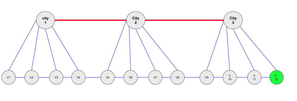
Let’s say you live in France, in the city of Paris, and you want to reach a small village V near Marseille. You basically have two kinds of roads in France:

• Highways that connect major cities together: these roads are fast and smooth (130 km/h) but not very dense.
• Smaller national roads connecting towns and villages: they’re slow, but very dense.

Now, imagine you don’t have Google Maps. What strategy would you use?
I think you already guessed it: the fastest strategy is to take the highway until the closest big city near the village, then switch to national roads to actually reach your destination.

Jokes aside, if you found that strategy, you’re going to understand the rest of this article just fine.

Technical Explanation:

In the classical world of databases, queries are supposed to return exact results. For example, if you have a relational database, the user might send a query that filters on a column, and if that column has an index, you can easily locate the rows with the target value.

The vector store world is a bit different: the user sends a vector (an embedding of a query), and our mission is to find vectors (embeddings) that are the closest to it. When you only have a few dozen vectors, you can scan them all and easily find the nearest match. But when you’re in a company with millions of vectors, it becomes much less obvious.

That’s where Approximate Nearest Neighbors (ANN) come in: a family of approximate search algorithms adapted to vector store databases. Within that family, there’s one algorithm that performs extremely well and will be the focus of this post: HNSW.

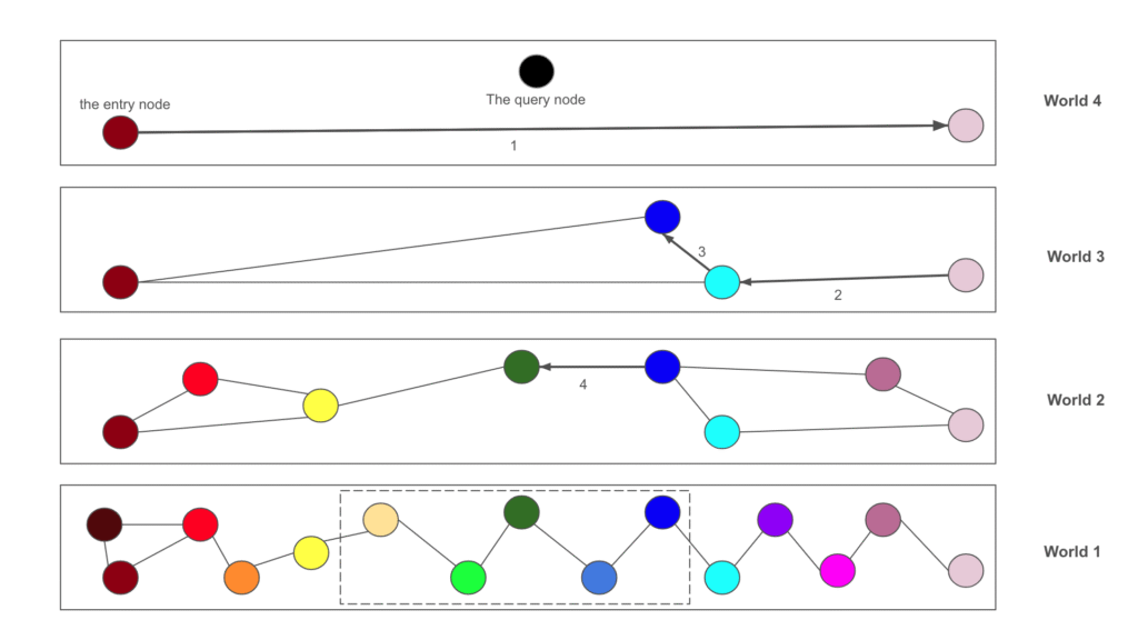
• Structure of the database:  As its name suggests, in HNSW the nodes are distributed across several hierarchical “small worlds.” You can think of it like a building with multiple floors: the higher the floor, the fewer nodes there are: The number of nodes decreases exponentially. Every node has a maximum level and appears on all levels below it. On each level, it is connected to its K nearest neighbors. Here is an example from the google colab where we have a database with 100K nodes distributed on 10 layers: 

--- Layers Density ---
Layer 0: 100000 nodes (100.00% of Total)
Layer 1: 74343 nodes (74.34% of Total)
Layer 2: 55421 nodes (55.42% of Total)
Layer 3: 41223 nodes (41.22% of Total)
Layer 4: 30760 nodes (30.76% of Total)
Layer 5: 22952 nodes (22.95% of Total)
Layer 6: 17087 nodes (17.09% of Total)
Layer 7: 12782 nodes (12.78% of Total)
Layer 8: 9487 nodes (9.49% of Total)
Layer 9: 7117 nodes (7.12% of Total)

• Search:
  Let’s say we want to find the K nearest nodes to a given vector (the query):
  • We pick a random node on the highest level.
  • We navigate this level until we can’t find any node closer than the current one.
    
  • We take the closest node on this level, go down to the next level, and repeat the same process (navigate the level until we can’t find anything closer, then go down).
    
  • Once we reach the bottom level (which contains all nodes), we search for the closest nodes among M candidates.

• Parameters:
  • L: the number of levels

  • M: the max number of neighbors per node on each level. Higher M leads to a denser graph, better recall and accuracy, but slower search/build time.

  • efConstruction: the size of the dynamic list of nearest neighbors considered during the insertion of a new vector: Higher efConstruction and M lead to better (more accurate) graph construction, but slower build time.

• Insertion:
  Insertion works a bit like search.
  • We determine the node’s maximum level using the following formula.

layer= min(𝐿,⌊−log(random[0,1])⋅log(𝑀)⌋)

• • We traverse levels from top to bottom. For each level:

• • • We run a greedy search from the entry point to find the closest neighbors.
    • We insert the node into the level and connect it to its M closest neighbors. We also update the neighbors of the other nodes on that level.
      The closest neighbor becomes the entry point for the next level down.

3. Playing with the algorithm:

Let’s insert 20,000 random nodes and look at the performance compared to a full-scan search (where we parse all nodes and get exact result). The query is also computed randomly. Our simulator class will insert the random vectors and perform two searchs (we always return the k-3 neighbors)

• A search using HNSW
• A full scan search: It is slow but returns exact results.

HNSWSimulator(layers_count=7, M=4, ef_construction=20).simulate(nodes_count=20000)

HNSWSimulator(layers_count=7, M=4, ef_construction=20).simulate(nodes_count=20000)

Inserting vectors ...: 100%|██████████| 20000/20000 [00:07<00:00, 2657.04it/s]

--- Layers Density ---
Layer 0: 20000 nodes (100.00% of Total)
Layer 1: 9724 nodes (48.62% of Total)
Layer 2: 4714 nodes (23.57% of Total)
Layer 3: 2244 nodes (11.22% of Total)
Layer 4: 1104 nodes (5.52% of Total)
Layer 5: 556 nodes (2.78% of Total)
Layer 6: 270 nodes (1.35% of Total)
Results of search using HNSW: 
Search duration: 0.0006
3 closest Neighbors
- Node ID #13275: Distance =  7.9647)
- Node ID #13526: Distance =  17.2537)
- Node ID #17936: Distance =  18.9266)
==================================
Results of search using fulls scan search: 
Search duration: 0.2076
3 closest Neighbors
- Node ID #2039: Distance =  2.2819)
- Node ID #15496: Distance =  2.6419)
- Node ID #2400: Distance =  3.9643)

We see that the search is much faster that full-scan search, but the result is not that much good.  The distances which are found with full scan search are approximately five times better.

Let’s increase the size of M and efConstruction and check the search quality. HNSW should be performing better now.

HNSWSimulator(layers_count=7, M=20, ef_construction=500).simulate(nodes_count=20000)

HNSWSimulator(layers_count=7, M=20, ef_construction=500).simulate(nodes_count=20000)

Results of search using HNSW: 
Search duration: 0.0045
3 closest Neighbors
- Node ID #18541: Distance =  2.1932)
- Node ID #13638: Distance =  6.1484)
- Node ID #14428: Distance =  8.1288)
==================================
Results of search using fulls scan search: 
Search duration: 0.1545
3 closest Neighbors
- Node ID #18541: Distance =  2.1932)
- Node ID #7300: Distance =  2.9153)
- Node ID #12472: Distance =  3.0299)

Bingo, we see that we,  now, have much better (acceptable) accuracy, but we are 35 times faster with HNSW.

Let’s make now try something big. We will make a big dataset with 100000 nodes, 10 layers, M=30 and ef_construction = 100

HNSWSimulator(layers_count=10, M=30, ef_construction=100).simulate(nodes_count=100000)

HNSWSimulator(layers_count=10, M=30, ef_construction=100).simulate(nodes_count=100000)

Search duration: 0.0074
3 closest Neighbors
- Node ID #34003: Distance =  0.9588)
- Node ID #16300: Distance =  1.3662)
- Node ID #52601: Distance =  1.9778)
==================================
Results of search using fulls scan search: 
Search duration: 0.6644
3 closest Neighbors
- Node ID #34003: Distance =  0.9588)
- Node ID #16300: Distance =  1.3662)
- Node ID #52601: Distance =  1.9778)

Waouh !! HNSW is performing very well on both accuracy (we find the exact neighbors) and latency (90 times faster) on this big dataset.

Conclusion:

Thanks to its architecture, HNSW is an algorithm that performs extremely well for vector stores and basically makes the whole RAG world possible.